Quickstart: Using Tessera on a Single Sample
Source:vignettes/vignette_basic.Rmd
vignette_basic.RmdLibs
suppressPackageStartupMessages({
    library(tessera)

    ## Downstream analysis in Seurat V5
    library(Seurat)

    ## Plotting functions
    ## Not imported by Tessera
    library(ggplot2)
    library(ggthemes)
    library(viridis)
    library(patchwork)
})

fig.size <- function(h, w) {
    options(repr.plot.height = h, repr.plot.width = w)
}
Data
Small sample MERFISH dataset from Chen et al:
https://www.biorxiv.org/content/10.1101/2023.04.04.535379v1.abstract
data('tessera_warmup')
counts = tessera_warmup$counts
meta_data = tessera_warmup$meta_data
meta_vars_include = c('type')
fig.size(8, 8)
ggplot() +
    geom_point(data = meta_data, aes(X, Y, color = type)) +
    theme_void() +
    scale_color_tableau() +
    coord_sf(expand = FALSE) +
    NULL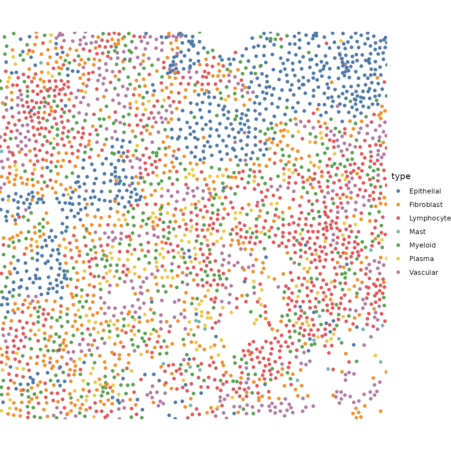
Some coarse grained cell types are predefined here, to help interpret the tiles we get below.
table(meta_data$type)
#>
#> Epithelial Fibroblast Lymphocyte       Mast    Myeloid     Plasma   Vascular
#>        634        588        829         18        491        206        411
Get Tiles
Run the Tessera algorithm to get tiles in one function. The result is returns in two structures:
- dmt: cell-level information.
- aggs: tile-level information.
The two are tied together through dmt$pts$agg_id
res = GetTiles(
    X = meta_data$X,
    Y = meta_data$Y,
    counts = counts,
    meta_data = meta_data,
    meta_vars_include = meta_vars_include,
)
#> Warning in GetTiles.default(X = meta_data$X, Y = meta_data$Y, counts = counts,
#> : No embeddings provided. Calculating embeddings using PCA.
#> Warning in GetTiles.default(X = meta_data$X, Y = meta_data$Y, counts = counts,
#> : No value for group.by provided. Analyzing as a single sample.
dmt = res$dmt
aggs = res$aggs
fig.size(10, 30)
purrr::map(1:3, function(i) {
    ggplot(cbind(aggs$meta_data, val=aggs$pcs[, i])) +
        geom_sf(aes(geometry = shape, fill = val)) +
        theme_void(base_size = 16) +
        coord_sf(expand = FALSE) +
        scale_fill_gradient2_tableau() +
        guides(color = 'none') +
        labs(title = paste0('PC', i)) +
        NULL
}) %>%
    purrr::reduce(`|`)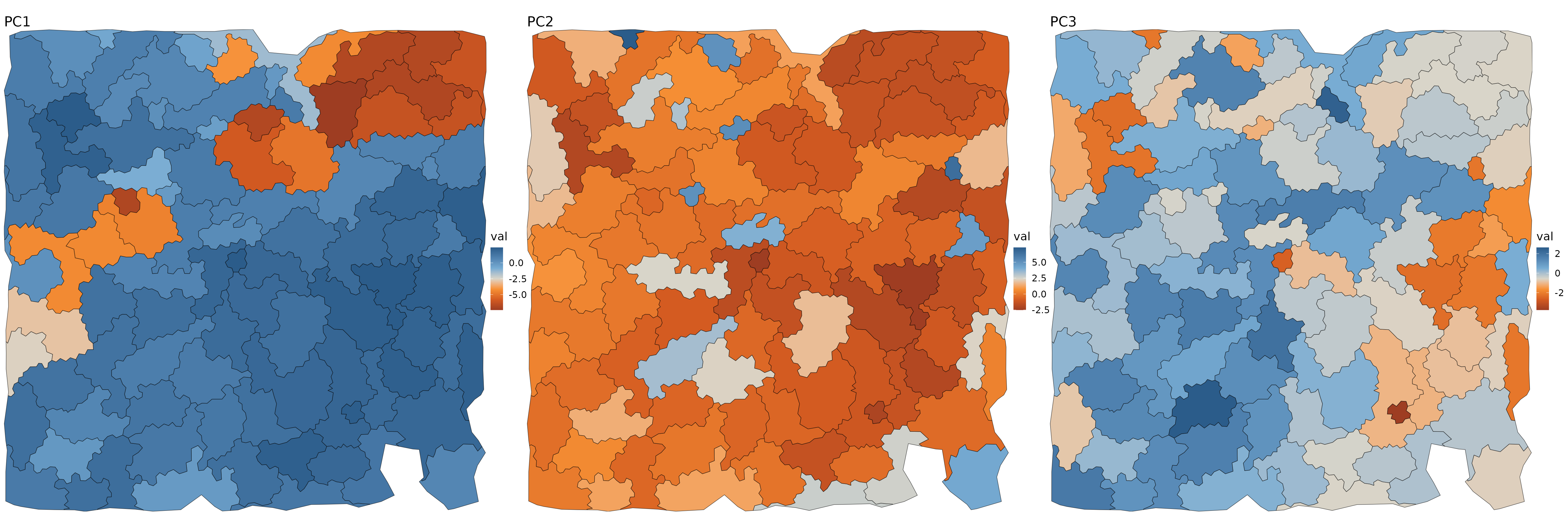
Cluster and label tiles
Let’s treat each aggregate as a unit of analysis.
obj = Seurat::CreateSeuratObject(
    counts = aggs$counts,
    meta.data = tibble::column_to_rownames(data.frame(dplyr::select(aggs$meta_data, -shape)), 'id')
)

## Seurat doesn't do sf shapes well
obj@meta.data$shape = aggs$meta_data$shape

## Represent each tile as the mean PC embeddings of all its cells
## NOTE: this tends to produce more biologically meaningful results than pooling gene counts per tile
rownames(aggs$pcs) = colnames(obj)
obj[['pca']] = Seurat::CreateDimReducObject(embeddings = aggs$pcs, loadings = dmt$udv_cells$loadings, key = 'pca_', assay = Seurat::DefaultAssay(obj))
Do all the typical steps for Seurat clustering.
.verbose = FALSE
obj = obj %>%
    NormalizeData(normalization.method = 'LogNormalize', scale.factor = median(obj@meta.data$nCount_RNA), verbose = .verbose) %>%
    RunUMAP(verbose = .verbose, dims = 1:10, reduction = 'pca') %>%
    Seurat::FindNeighbors(features = 1:10, reduction = 'pca', verbose = .verbose) %>%
    Seurat::FindClusters(verbose = .verbose, resolution = c(2))
#> Warning: The default method for RunUMAP has changed from calling Python UMAP via reticulate to the R-native UWOT using the cosine metric
#> To use Python UMAP via reticulate, set umap.method to 'umap-learn' and metric to 'correlation'
#> This message will be shown once per session
Let’s see the aggregate clusters in UMAP and physical space.
p1 = DimPlot(obj, reduction = 'umap', group.by = 'seurat_clusters') + scale_color_tableau('Classic 10')
p2 = ggplot(obj@meta.data) +
    geom_sf(aes(geometry = shape, fill = seurat_clusters)) +
    theme_void(base_size = 16) +
    coord_sf(expand = FALSE) +
    scale_fill_tableau('Classic 10') +
    NULL

fig.size(6, 12)
(p1 | p2) + plot_layout(widths = c(1, 1))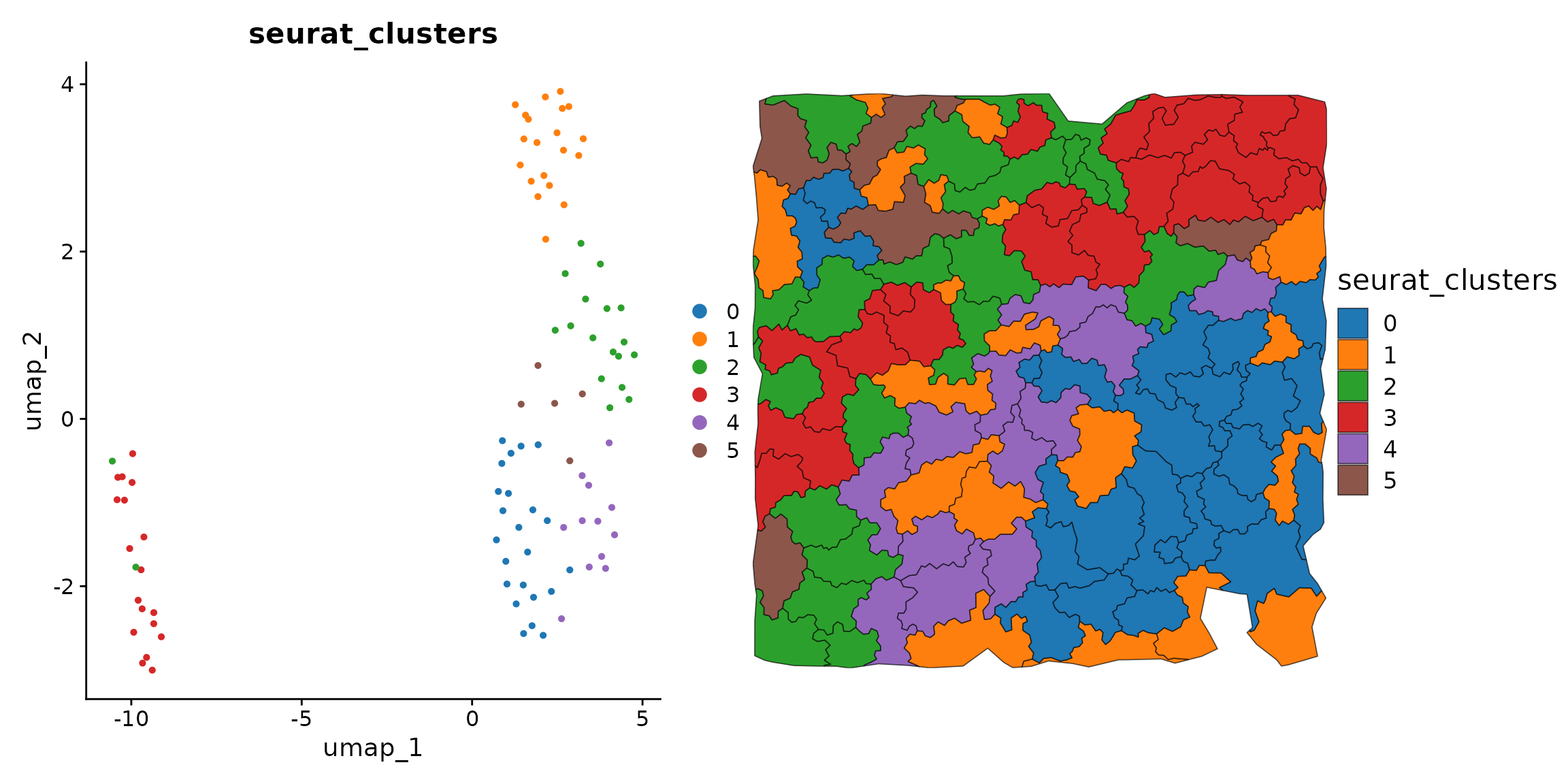
Transfer agg information to cells
dmt$pts$spatial_cluster = obj@meta.data$seurat_clusters[dmt$pts$agg_id]
p1 = ggplot() +
    geom_sf(data = obj@meta.data, aes(geometry = shape), fill = NA) +
    geom_point(data = dmt$pts, aes(X, Y, color = type)) +
    scale_color_tableau() +
    theme_void() +
    coord_sf(expand = FALSE) +
    NULL
p2 = ggplot() +
    geom_sf(data = obj@meta.data, aes(geometry = shape, fill = seurat_clusters), alpha = .2) +
    geom_point(data = dmt$pts, aes(X, Y, color = spatial_cluster)) +
    scale_color_tableau('Classic 10') +
    scale_fill_tableau('Classic 10') +
    theme_void() +
    guides(fill = 'none') +
    coord_sf(expand = FALSE) +
    NULL
fig.size(8, 20)
p1 | p2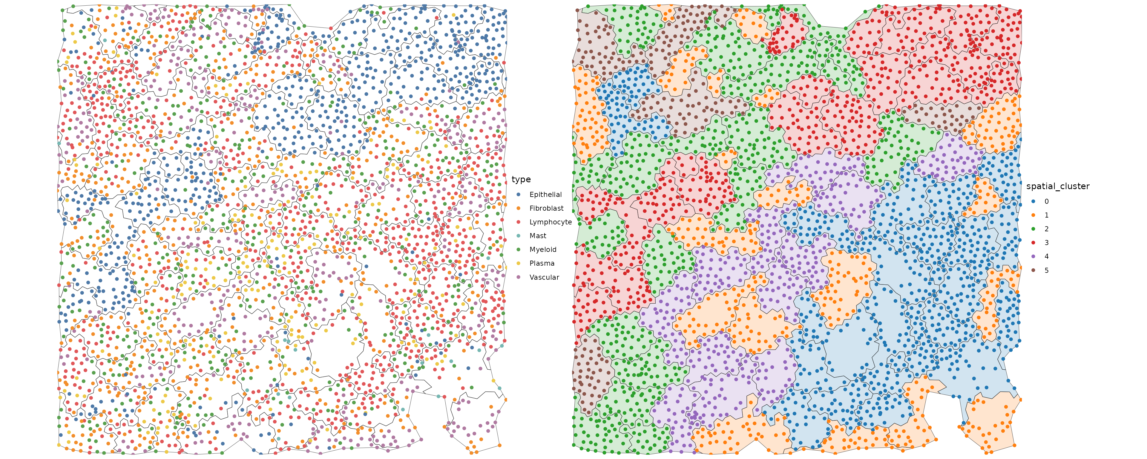
Let’s look at the composition of the spatial clusters.
fig.size(8, 10)
dmt$pts %>%
    with(table(type, spatial_cluster)) %>%
    prop.table(2) %>%
    data.table() %>%
    ggplot(aes(spatial_cluster, 100 * N, fill = type)) +
        geom_bar(stat = 'identity', position = position_stack()) +
        scale_fill_tableau() +
        theme_bw(base_size = 20) +
        labs(y = '% of spatial cluster', fill = 'cell type') +
        NULL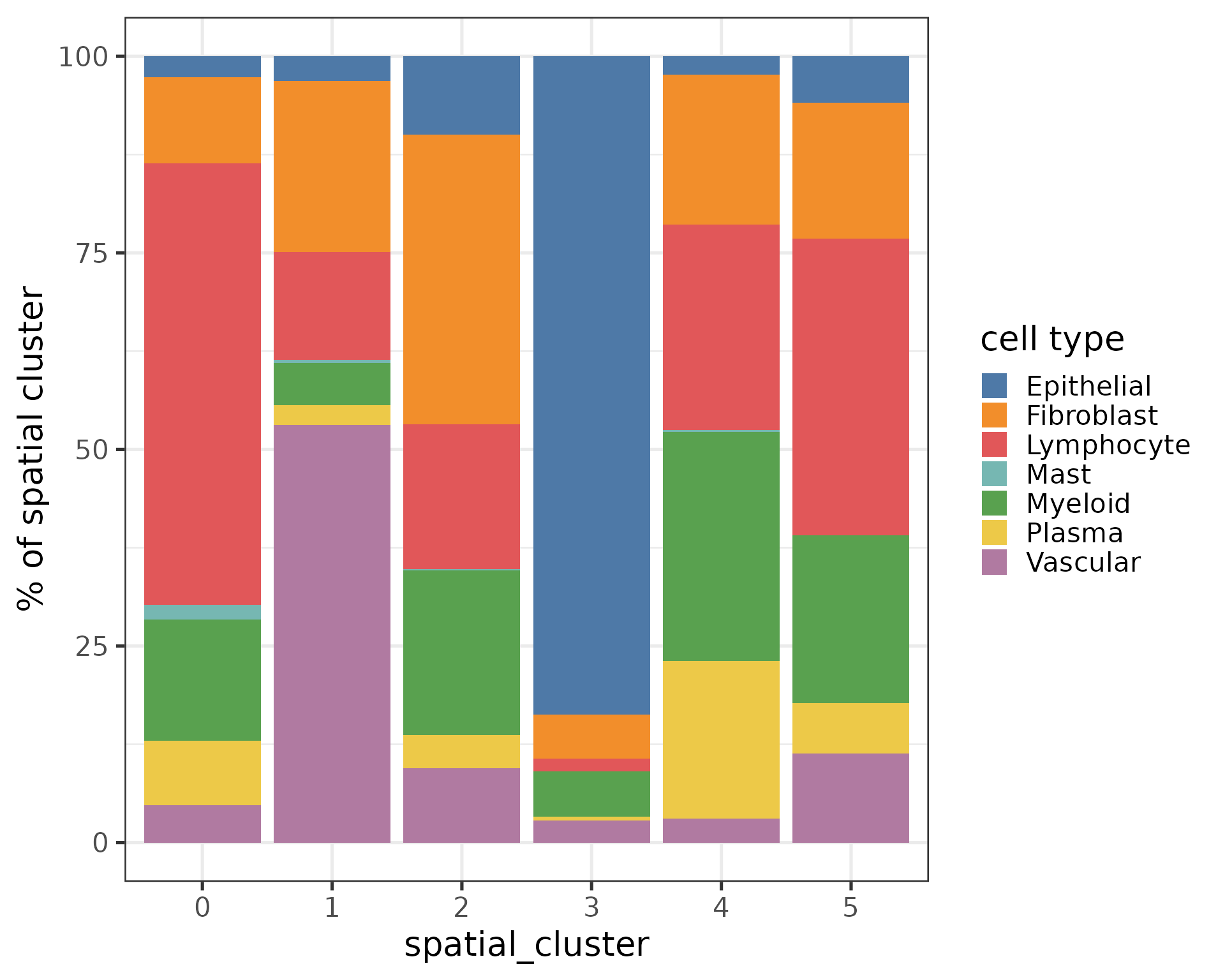
We can also query genes in space as we usually do in cells.
feature = 'MKI67' ## dividing cells
# feature = 'CD3E' ## T cells

fig.size(8, 10)
ggplot() +
    geom_sf(data = cbind(obj@meta.data, FetchData(obj, feature)), aes(geometry = shape, fill = !!sym(feature))) +
    scale_fill_gradient(low = 'white', high = '#832424') +
    theme_void() +
    coord_sf(expand = FALSE) +
    NULL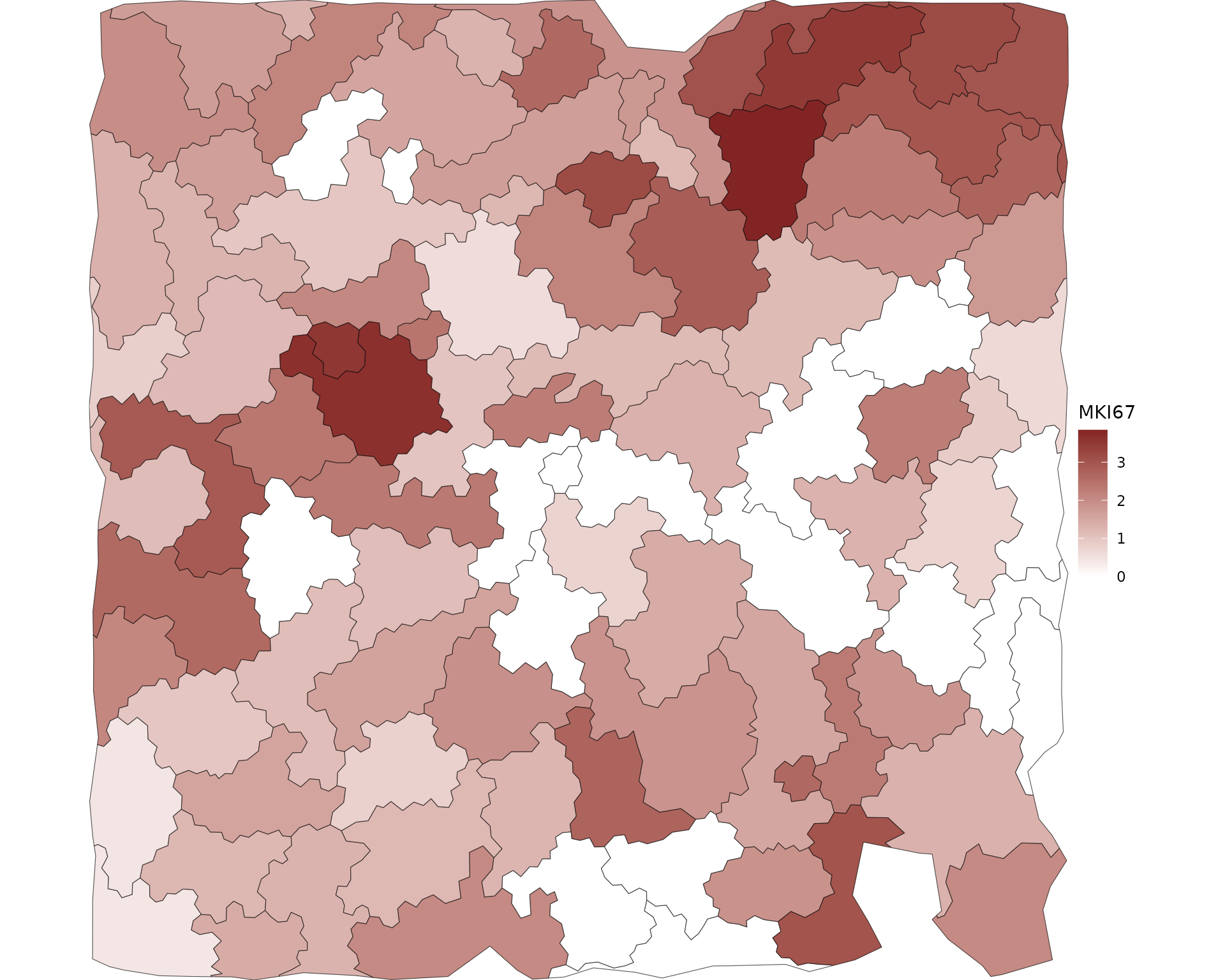
Session Info
sessionInfo()
#> R version 4.5.2 (2025-10-31)
#> Platform: x86_64-pc-linux-gnu
#> Running under: Ubuntu 24.04.3 LTS
#>
#> Matrix products: default
#> BLAS:   /usr/lib/x86_64-linux-gnu/openblas-pthread/libblas.so.3
#> LAPACK: /usr/lib/x86_64-linux-gnu/openblas-pthread/libopenblasp-r0.3.26.so;  LAPACK version 3.12.0
#>
#> locale:
#>  [1] LC_CTYPE=C.UTF-8       LC_NUMERIC=C           LC_TIME=C.UTF-8
#>  [4] LC_COLLATE=C.UTF-8     LC_MONETARY=C.UTF-8    LC_MESSAGES=C.UTF-8
#>  [7] LC_PAPER=C.UTF-8       LC_NAME=C              LC_ADDRESS=C
#> [10] LC_TELEPHONE=C         LC_MEASUREMENT=C.UTF-8 LC_IDENTIFICATION=C
#>
#> time zone: UTC
#> tzcode source: system (glibc)
#>
#> attached base packages:
#> [1] stats     graphics  grDevices utils     datasets  methods   base
#>
#> other attached packages:
#>  [1] purrr_1.2.1        future_1.68.0      patchwork_1.3.2    viridis_0.6.5
#>  [5] viridisLite_0.4.2  ggthemes_5.2.0     ggplot2_4.0.1      Seurat_5.4.0
#>  [9] SeuratObject_5.3.0 sp_2.2-0           tessera_0.1.10     Rcpp_1.1.1
#> [13] data.table_1.18.0
#>
#> loaded via a namespace (and not attached):
#>   [1] RColorBrewer_1.1-3     jsonlite_2.0.0         magrittr_2.0.4
#>   [4] spatstat.utils_3.2-1   farver_2.1.2           rmarkdown_2.30
#>   [7] fs_1.6.6               ragg_1.5.0             vctrs_0.6.5
#>  [10] ROCR_1.0-11            spatstat.explore_3.6-0 htmltools_0.5.9
#>  [13] sass_0.4.10            sctransform_0.4.3      parallelly_1.46.1
#>  [16] KernSmooth_2.23-26     bslib_0.9.0            htmlwidgets_1.6.4
#>  [19] desc_1.4.3             ica_1.0-3              plyr_1.8.9
#>  [22] plotly_4.11.0          zoo_1.8-15             cachem_1.1.0
#>  [25] igraph_2.2.1           mime_0.13              lifecycle_1.0.5
#>  [28] pkgconfig_2.0.3        Matrix_1.7-4           R6_2.6.1
#>  [31] fastmap_1.2.0          magic_1.6-1            fitdistrplus_1.2-4
#>  [34] shiny_1.12.1           digest_0.6.39          furrr_0.3.1
#>  [37] tensor_1.5.1           RSpectra_0.16-2        irlba_2.3.5.1
#>  [40] textshaping_1.0.4      labeling_0.4.3         progressr_0.18.0
#>  [43] spatstat.sparse_3.1-0  httr_1.4.7             polyclip_1.10-7
#>  [46] abind_1.4-8            compiler_4.5.2         proxy_0.4-29
#>  [49] withr_3.0.2            S7_0.2.1               DBI_1.2.3
#>  [52] fastDummies_1.7.5      MASS_7.3-65            classInt_0.4-11
#>  [55] tools_4.5.2            units_1.0-0            lmtest_0.9-40
#>  [58] otel_0.2.0             httpuv_1.6.16          future.apply_1.20.1
#>  [61] goftest_1.2-3          glue_1.8.0             nlme_3.1-168
#>  [64] promises_1.5.0         grid_4.5.2             sf_1.0-24
#>  [67] Rtsne_0.17             cluster_2.1.8.1        reshape2_1.4.5
#>  [70] generics_0.1.4         gtable_0.3.6           spatstat.data_3.1-9
#>  [73] class_7.3-23           tidyr_1.3.2            spatstat.geom_3.6-1
#>  [76] RcppAnnoy_0.0.23       ggrepel_0.9.6          RANN_2.6.2
#>  [79] pillar_1.11.1          stringr_1.6.0          spam_2.11-3
#>  [82] RcppHNSW_0.6.0         later_1.4.5            splines_4.5.2
#>  [85] dplyr_1.1.4            lattice_0.22-7         survival_3.8-3
#>  [88] deldir_2.0-4           tidyselect_1.2.1       miniUI_0.1.2
#>  [91] pbapply_1.7-4          knitr_1.51             gridExtra_2.3
#>  [94] scattermore_1.2        xfun_0.55              matrixStats_1.5.0
#>  [97] stringi_1.8.7          lazyeval_0.2.2         yaml_2.3.12
#> [100] evaluate_1.0.5         codetools_0.2-20       tibble_3.3.1
#> [103] cli_3.6.5              uwot_0.2.4             geometry_0.5.2
#> [106] xtable_1.8-4           reticulate_1.44.1      systemfonts_1.3.1
#> [109] jquerylib_0.1.4        globals_0.18.0         spatstat.random_3.4-3
#> [112] png_0.1-8              spatstat.univar_3.1-5  parallel_4.5.2
#> [115] pkgdown_2.2.0          dotCall64_1.2          mclust_6.1.2
#> [118] listenv_0.10.0         scales_1.4.0           e1071_1.7-17
#> [121] ggridges_0.5.7         rlang_1.1.7            cowplot_1.2.0