Walkthrough: Tessera Algorithm Step-by-Step
Source:vignettes/vignette_stepthrough.Rmd
vignette_stepthrough.RmdOverview
This notebook is a walkthrough of the steps of Tessera, for those who want to get more familiar with the components.
Parameters
verbose = TRUE
show_plots = TRUE

###### STEP 0 ######
npcs = 10
## Graph pruning
prune_thresh_quantile = 0.95
prune_min_cells = 10


###### STEP 1: GRADIENTS ######
smooth_distance = c('none', 'euclidean', 'projected', 'constant')[3]
smooth_similarity = c('none', 'euclidean', 'projected', 'constant')[3]


###### STEP 2: DMT ######
## ... no options


###### STEP 3: AGGREGATION ######
max_npts = 50
min_npts = 5
alpha = 1 ## 0.2 = conservative merging, 2 = liberal merging
Data
Small sample MERFISH dataset from Chen et al:
https://www.biorxiv.org/content/10.1101/2023.04.04.535379v1.abstract
data('tessera_warmup')
counts = tessera_warmup$counts
meta_data = tessera_warmup$meta_data
meta_vars_include = c('type')
fig.size(8, 8)
ggplot() +
    geom_point(data = meta_data, aes(X, Y, color = type)) +
    theme_void() +
    scale_color_tableau() +
    coord_sf(expand = FALSE) +
    NULL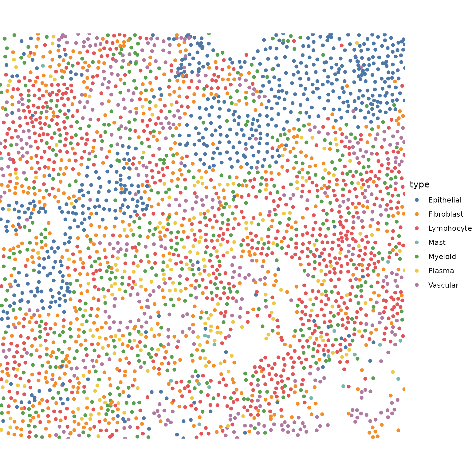
Some coarse and fine grained cell types are predefined here, to help interpret the tiles we get below.
table(meta_data$type)
#>
#> Epithelial Fibroblast Lymphocyte       Mast    Myeloid     Plasma   Vascular
#>        634        588        829         18        491        206        411
prepare
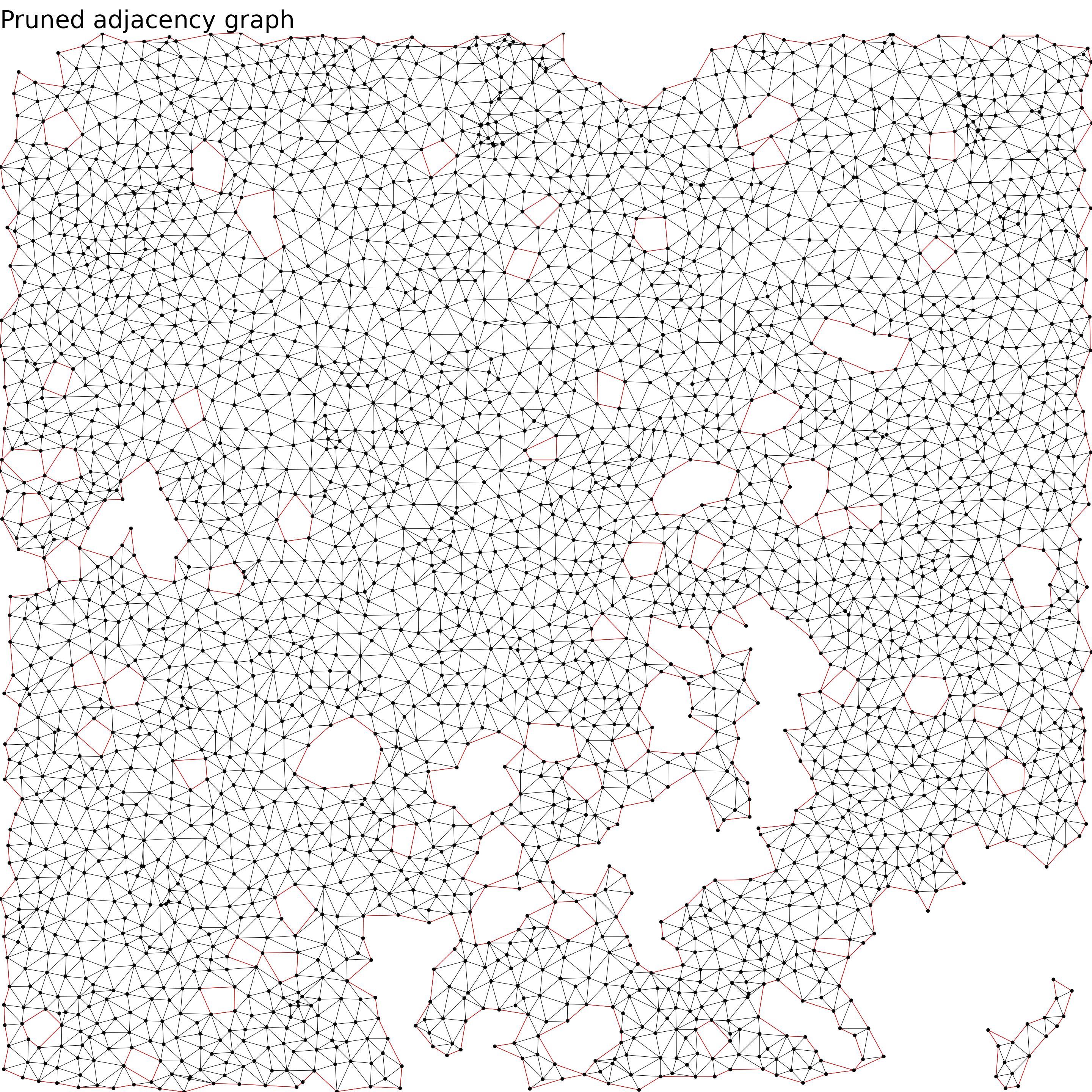
dmt = init_data(meta_data$X, meta_data$Y, counts, meta_data, meta_vars_include)
dmt = prune_graph(dmt, thresh_quantile = prune_thresh_quantile, mincells = prune_min_cells)
dmt = add_exterior_triangles(dmt)
fig.size(15, 15)
# fig.size(20, 20)

if (show_plots) {
    ggplot() +

        # ## big data
        # geom_point(data = dmt$pts, aes(X, Y), shape = '.', alpha = .1) +
        # geom_segment(data = dmt$edges[boundary == TRUE], aes(x = x0_pt, y = y0_pt, xend = x1_pt, yend = y1_pt), color = 'red', lwd = .2) +

        ## small data
        geom_segment(data = dmt$edges, aes(x = x0_pt, y = y0_pt, xend = x1_pt, yend = y1_pt), color = 'black', lwd = .2) +
        geom_segment(data = dmt$edges[boundary == TRUE], aes(x = x0_pt, y = y0_pt, xend = x1_pt, yend = y1_pt), color = 'red', lwd = .2) +
        geom_point(data = dmt$pts, aes(X, Y), size = .5) +

        theme_void(base_size = 20) +
        coord_cartesian(expand = FALSE) +
        labs(title = 'Pruned adjacency graph') +
        NULL
}
pca
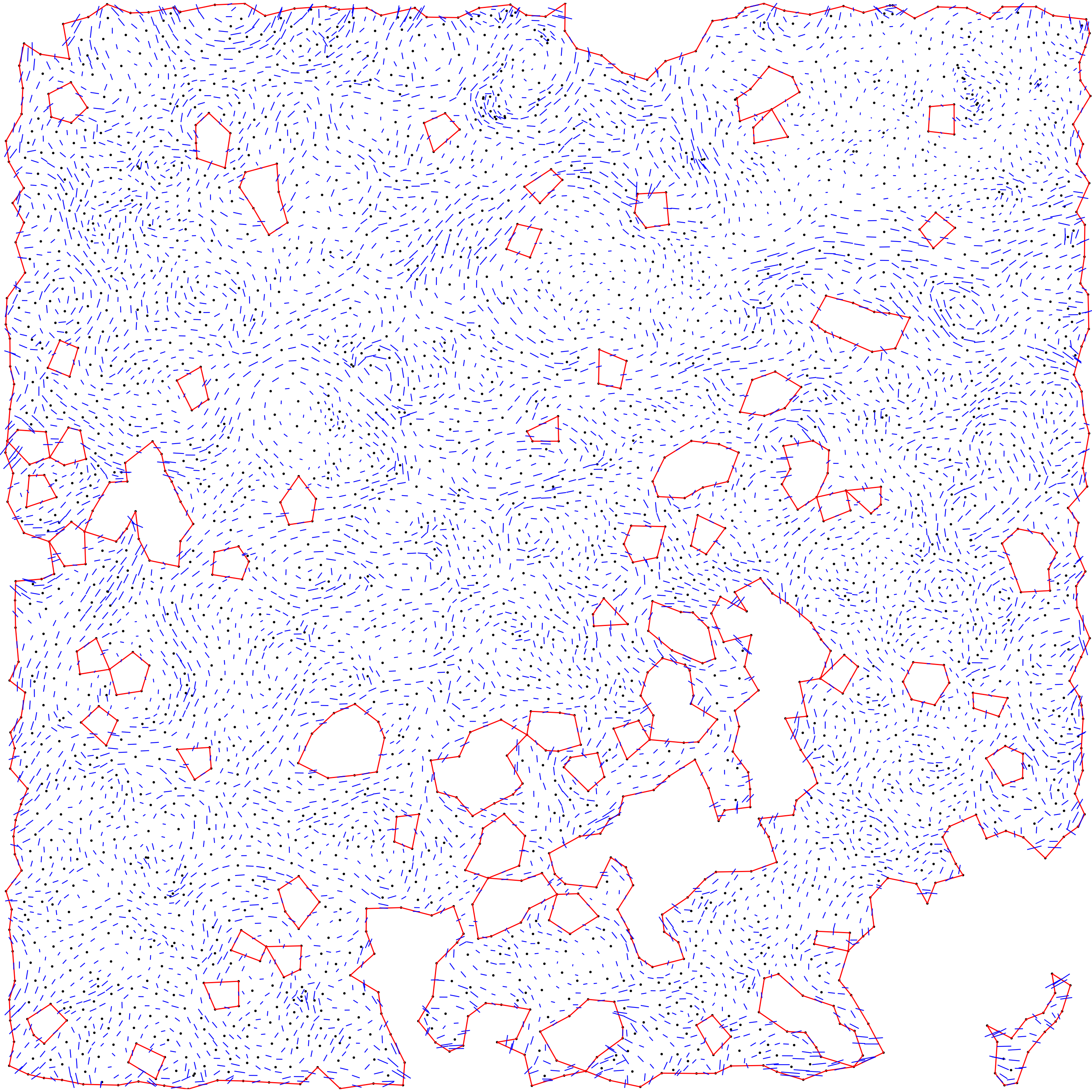
dmt$udv_cells = do_pca(dmt$counts, npcs)Step 1: compute gradients on all data structures
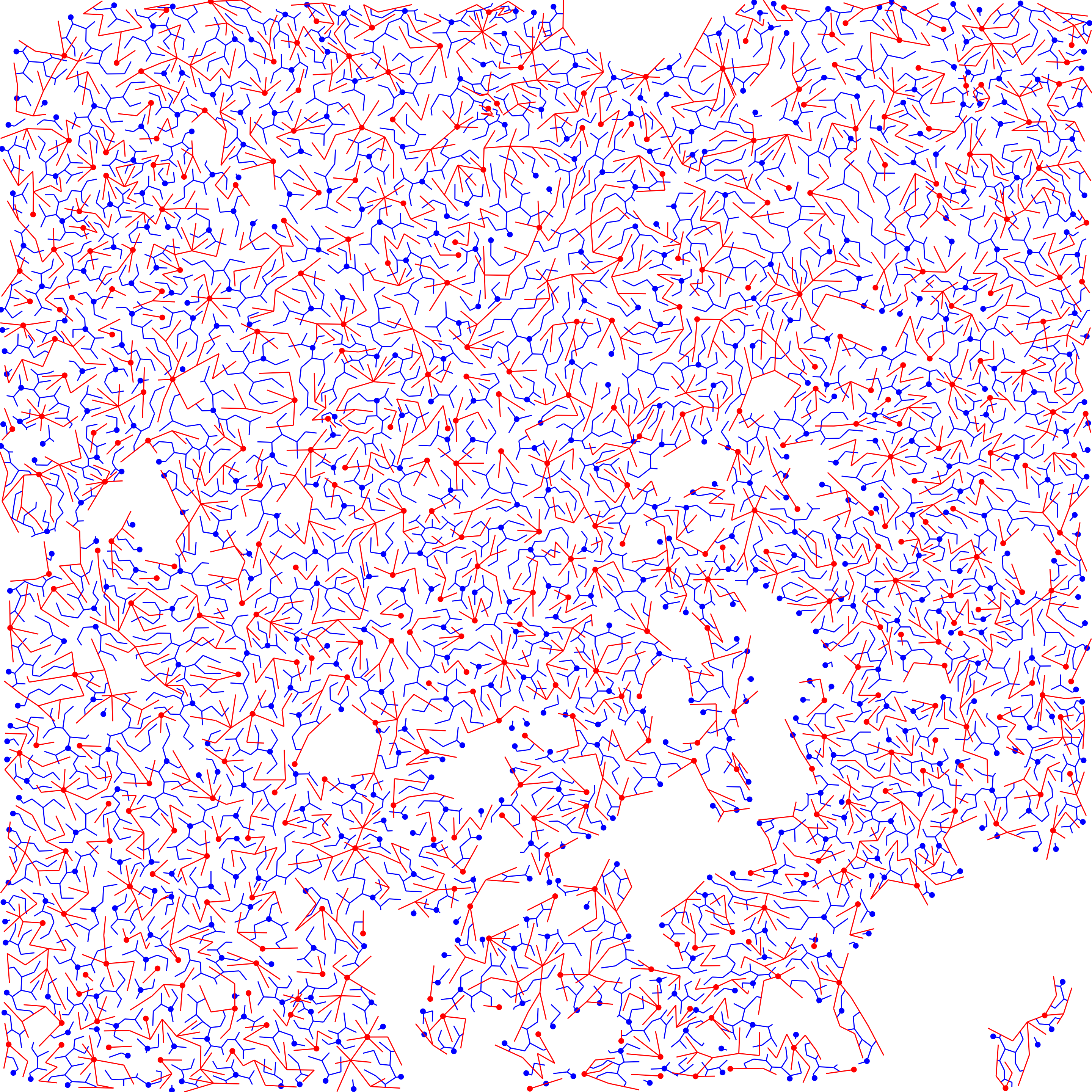
field = compute_gradients(dmt, smooth_distance, smooth_similarity)
field = compress_gradients_svd(field)
if (show_plots) {

    len_plot_constant = .8
    fig.size(15, 15)
    # fig.size(20, 20)
    ggplot() +
        geom_point(data = dmt$pts, aes(X, Y), size = .5) +
        geom_segment(data = dmt$edges[boundary == TRUE, ], aes(x = x0_pt, y = y0_pt, xend = x1_pt, yend = y1_pt), color = 'red') +

        ## Triangle Gradients
        geom_segment(
            data = data.table(dmt$tris, field$tris_svd),
            aes(
                x=X-len_plot_constant*(len_grad+len_ortho)*dx_ortho,
                y=Y-len_plot_constant*(len_grad+len_ortho)*dy_ortho,
                xend=X+len_plot_constant*(len_grad+len_ortho)*dx_ortho,
                yend=Y+len_plot_constant*(len_grad+len_ortho)*dy_ortho
            ),
            linewidth = .4, alpha = 1,
            color = 'blue'
        ) +

        theme_void() +
        coord_fixed(expand = FALSE) +
        NULL
}
Step 2: DMT
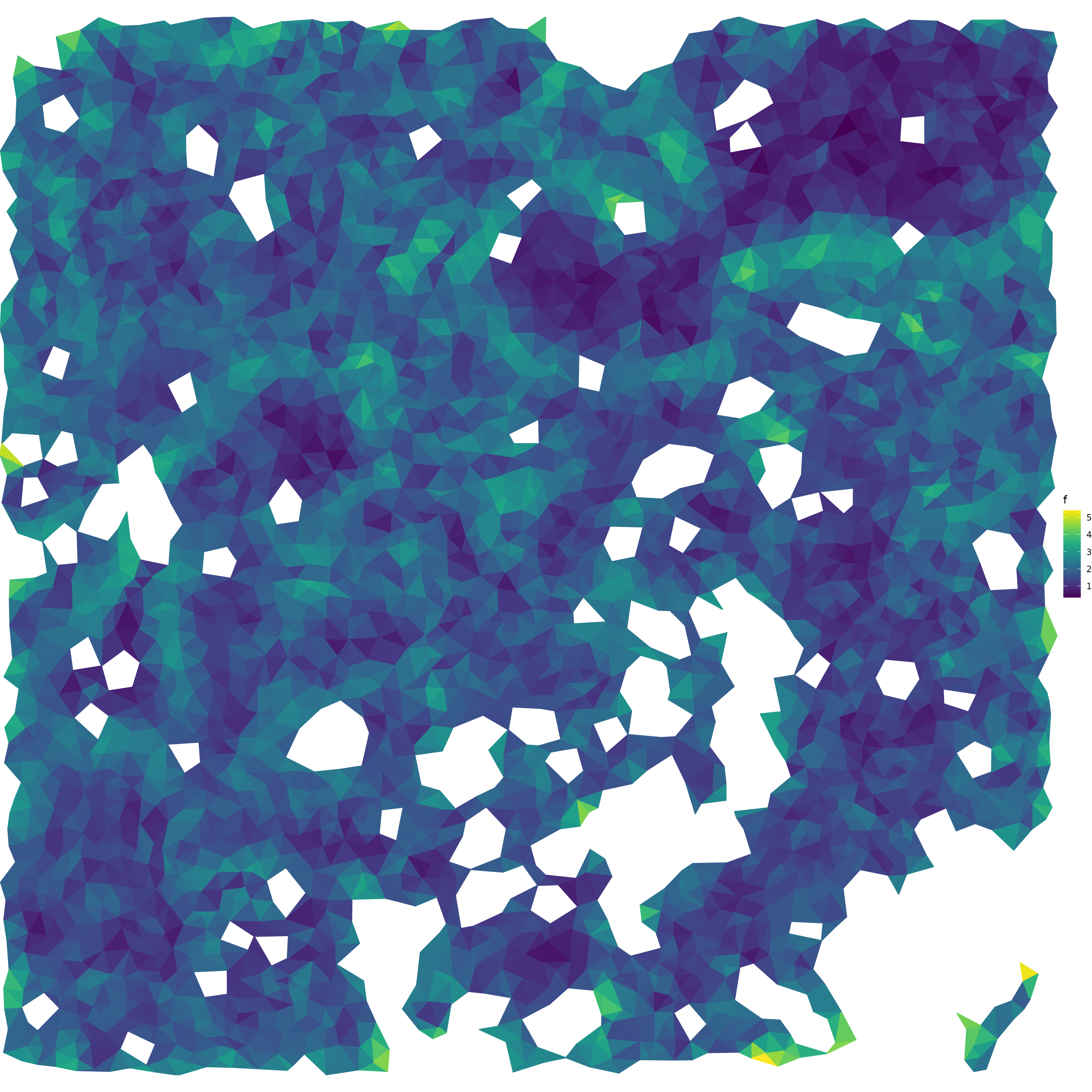
compute f
dmt = dmt_set_f(dmt, field)
if (show_plots) {
    ntri = max(which(dmt$tris$external == FALSE))
    i = Matrix::t(dmt$tri_to_pt[1:ntri, ])@i+1
    plt_df = data.table(
        X = dmt$pts$X[i],
        Y = dmt$pts$Y[i],
        f = rep(dmt$tris$f[1:ntri], each = 3)
    )[
        , id := rep(1:ntri, each = 3)
    ][]


    fig.size(15, 15)
    ggplot() +
        geom_polygon(data = plt_df, aes(X, Y, group = id, fill = f, color = f)) +
        theme_void() +
        coord_fixed(expand = FALSE) +
        scale_fill_viridis() +
        scale_color_viridis() +
        NULL
}
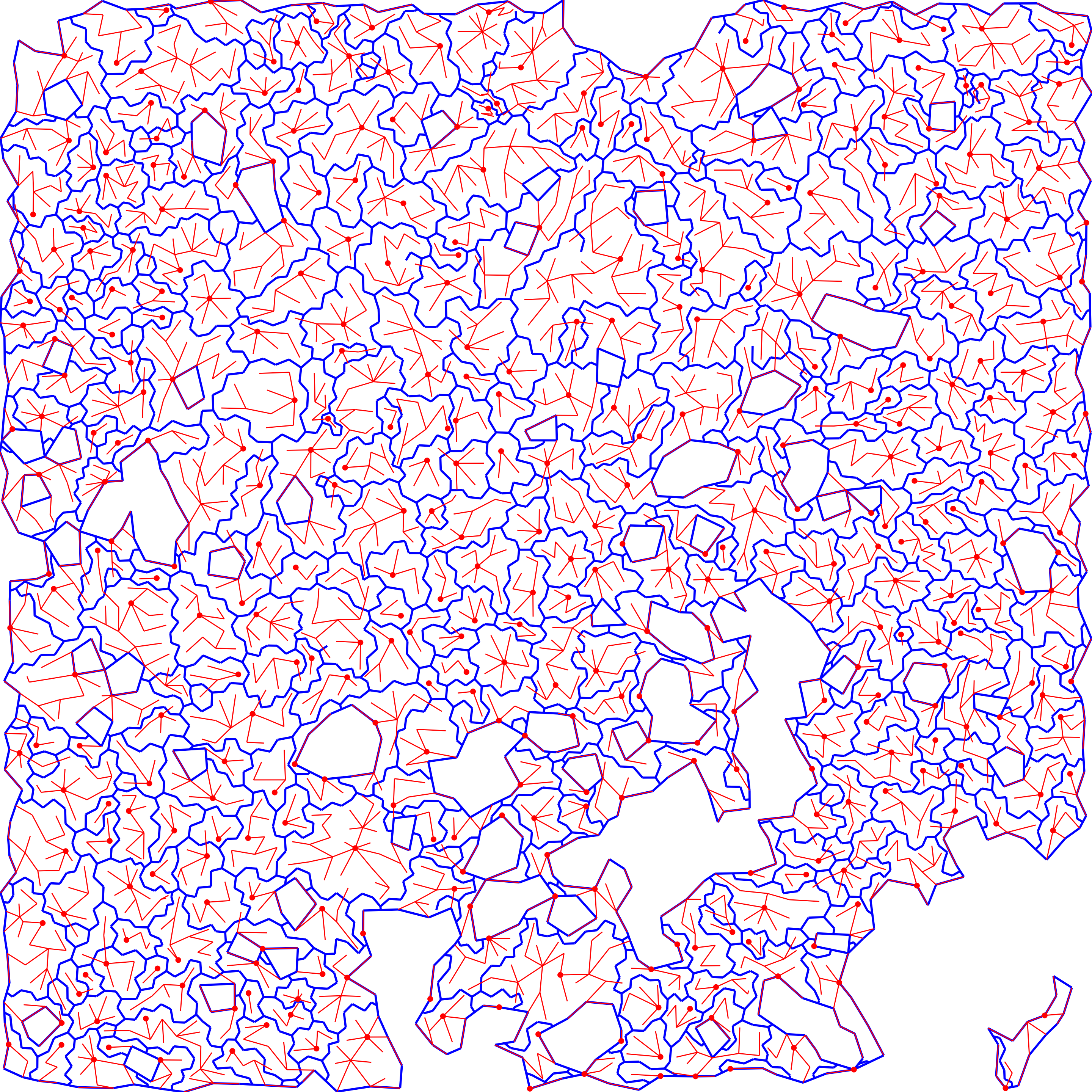
forests
dmt$prim = do_primary_forest(dmt)
dmt$dual = do_dual_forest(dmt)
if (show_plots) {
    fig.size(15, 15)
    ggplot() +
        ## primary forest
        geom_point(data = dmt$tris[dmt$dual$maxima, ], aes(X, Y), color = 'blue', size = 2) +
        geom_segment(data = dmt$dual$edges, aes(x=x0, y=y0, xend=x1, yend=y1), color = 'blue') +

        ## primary forest
        geom_point(data = dmt$pts[dmt$prim$minima, ], aes(X, Y), color = 'red', size = 2) +
        geom_segment(data = dmt$prim$edges, aes(x=x0, y=y0, xend=x1, yend=y1), color = 'red') +

        theme_void() +
        coord_cartesian(expand = FALSE) +
        NULL
}
extract epaths
dmt$e_sep = dmt_get_separatrices(dmt)After DMT, we have a separatrix (in blue) and the primary forest connecting points (in red).
if (show_plots) {
    fig.size(15, 15)
    ggplot() +

        geom_segment(data = dmt$edges[dmt$e_sep, ], aes(x = x0_tri, y = y0_tri, xend = x1_tri, yend = y1_tri), lwd = 1, color = 'blue') +
        geom_segment(data = dmt$edges[boundary == TRUE], aes(x = x0_pt, y = y0_pt, xend = x1_pt, yend = y1_pt), color = 'blue', lwd = 1) +

        ## primary forest
        geom_point(data = dmt$pts[dmt$prim$minima, ], aes(X, Y), color = 'red', size = 2) +
        geom_segment(data = dmt$prim$edges, aes(x=x0, y=y0, xend=x1, yend=y1), color = 'red') +

        theme_void() +
        coord_cartesian(expand = FALSE) +
        NULL
}
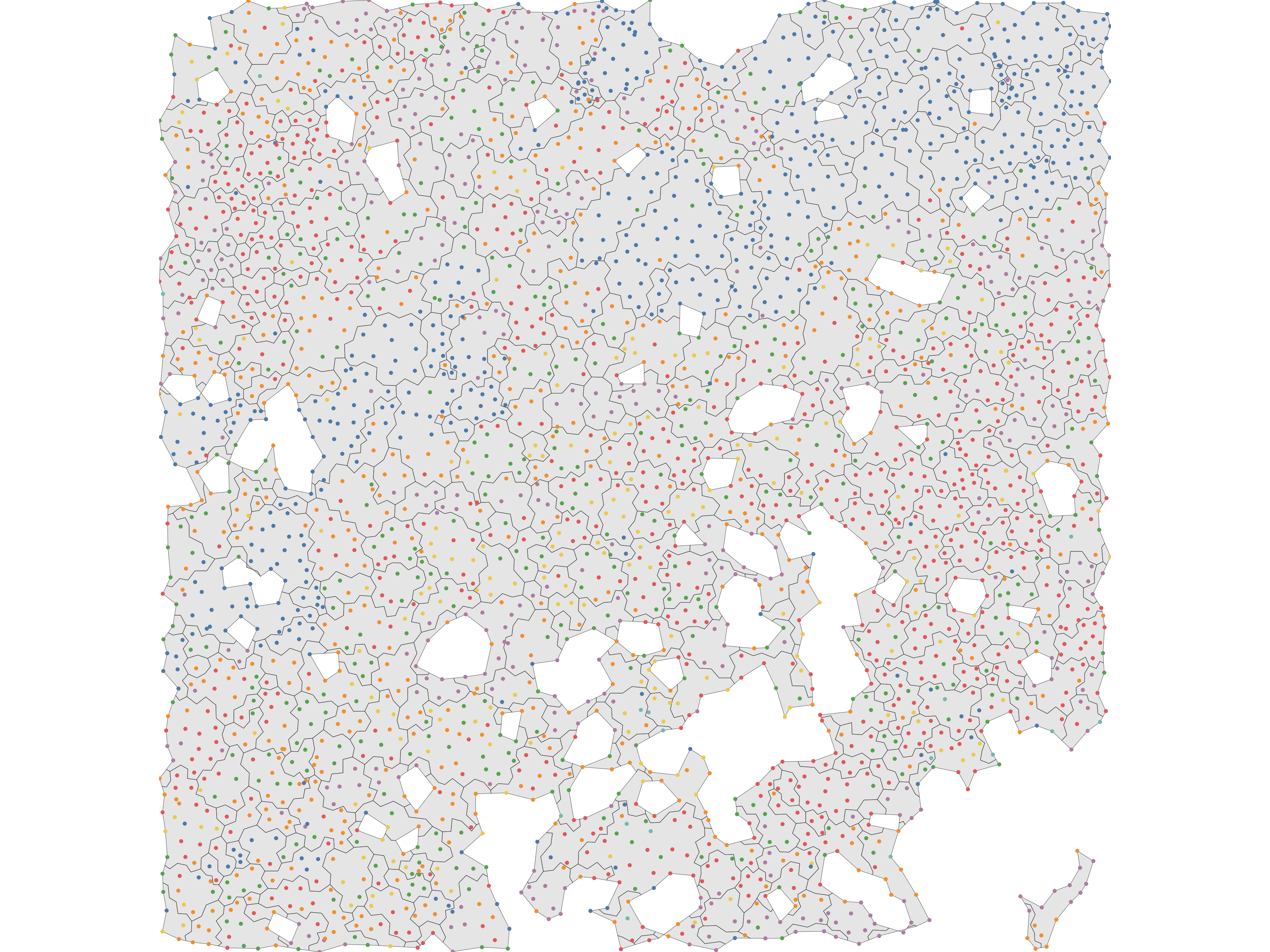
extract tiles
dmt = dmt_assign_tiles(dmt)
aggs = dmt_init_tiles(dmt)
if (show_plots) {
    set.seed(2)
    fig.size(15, 20)
    ggplot() +
        geom_sf(data = aggs$meta_data$shape) +
        # geom_point(data = dmt$pts, aes(X, Y, color = factor(agg_id, sample(nrow(aggs$meta_data)))), size = 1) +
        # scale_color_tableau() +
        theme_void() +
        coord_sf(expand = FALSE) +
        # coord_cartesian(expand = FALSE) +
        guides(color = 'none') +

        NULL
}
if (show_plots) {
    set.seed(2)
    fig.size(15, 20)
    ggplot() +
        geom_sf(data = aggs$meta_data$shape) +
        geom_point(data = dmt$pts, aes(X, Y, color = type)) +
        theme_void() +
        coord_sf(expand = FALSE) +
        scale_color_tableau() +
        guides(color = 'none') +
        NULL
}
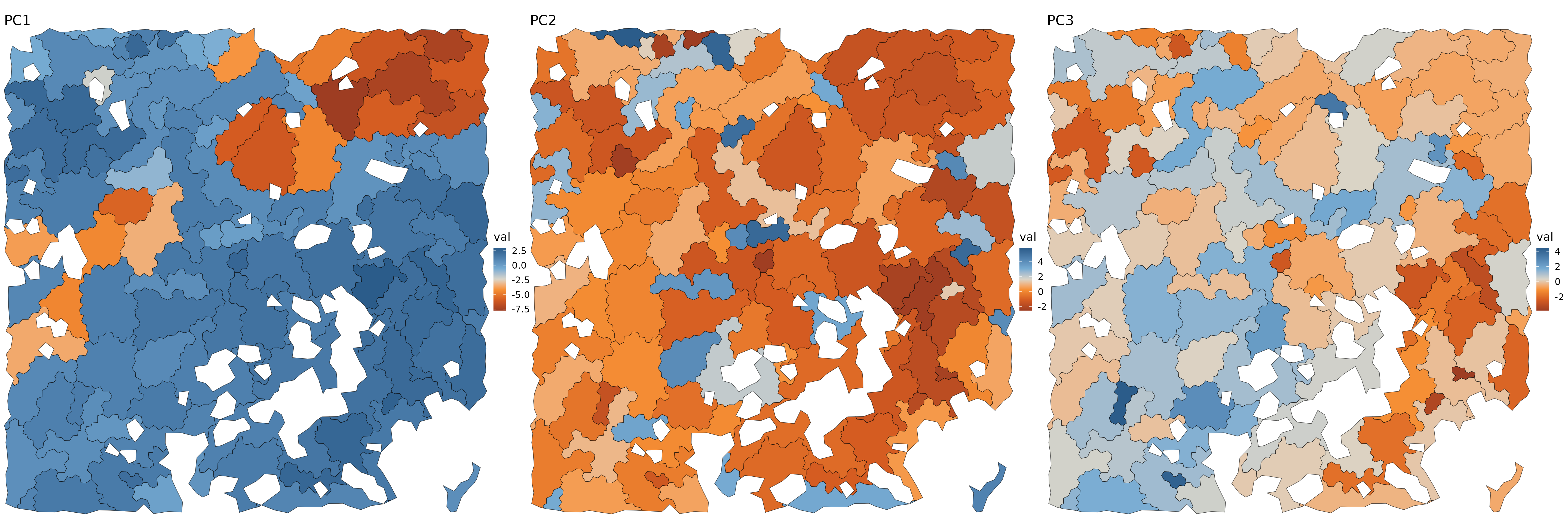
Step 3: Aggregation
Merge main
First, merge similar aggregates that are nearby.
aggs = init_scores(aggs, agg_mode=2, alpha=alpha, max_npts=max_npts)
aggs = merge_aggs(aggs, agg_mode=2, max_npts=max_npts)
dmt = update_dmt_aggid(dmt, aggs)
aggs = update_agg_shapes(dmt, aggs)
Merge small outliers
Then go ahead and merge small clusters that are smaller than
aggs = init_scores(aggs, agg_mode=3, alpha=alpha, min_npts=min_npts)
aggs = merge_aggs(aggs, agg_mode=3, min_npts=min_npts)
dmt = update_dmt_aggid(dmt, aggs)
aggs = update_agg_shapes(dmt, aggs)
Final tiles
fig.size(10, 30)
if (show_plots) {
    purrr::map(1:3, function(i) {
        ggplot(cbind(aggs$meta_data, val=aggs$pcs[, i])) +
            geom_sf(aes(geometry = shape, fill = val)) +
            theme_void(base_size = 16) +
            coord_sf(expand = FALSE) +
            scale_fill_gradient2_tableau() +
            guides(color = 'none') +
            labs(title = paste0('PC', i)) +
            NULL
    }) %>%
        purrr::reduce(`|`)
}
Results
Aggregates
The primary output is the tiles. Each tile has a row in the meta_data table:
- npts denotes the number of cells in the tile.
head(aggs$meta_data)
#>       id        X        Y  npts                          shape      area
#>    <int>    <num>    <num> <num>                 <sfc_GEOMETRY>     <num>
#> 1:     1 5578.221 10074.77    39 POLYGON ((5598.428 10051.98... 2624.2586
#> 2:     2 5523.750 10051.83    43 POLYGON ((5513.932 10008.66... 2718.7684
#> 3:     3 5550.940 10103.57    36 POLYGON ((5572.969 10116.07... 2405.4418
#> 4:     4 5577.735 10114.87     8 POLYGON ((5572.969 10116.07...  651.2121
#> 5:     5 5565.044 10019.62    41 POLYGON ((5614.379 10006.3,... 2292.7048
#> 6:     6 5609.770 10088.19    14 POLYGON ((5631.174 10097.96...  998.8177
#>    perimeter
#>        <num>
#> 1:  428.9675
#> 2:  305.5045
#> 3:  281.2410
#> 4:  139.6050
#> 5:  317.2784
#> 6:  189.5318
We also have pooled gene counts, for differential gene expression analysis.
aggs$counts[1:5, 1:5]
#> 5 x 5 sparse Matrix of class "dgCMatrix"
#>       1 2 3 4 5
#> ACE   1 2 2 1 1
#> ACKR1 . . 1 . .
#> ACKR2 1 . . . .
#> ACKR3 . . 1 . 1
#> ACKR4 . 2 . . .
And we have PCA embeddings for the tiles.
head(aggs$pcs)
#>            PC1        PC2         PC3        PC4       PC5         PC6
#> [1,] 0.6254406  1.0283725  0.83291401 -1.8056105 0.7110007 -0.03214636
#> [2,] 0.5616029 -0.2555397  0.42623300 -1.0095698 0.5037828  0.40149483
#> [3,] 1.2233199 -0.4752796  1.14695964 -0.6278043 0.8871260 -0.06488547
#> [4,] 1.3895474 -1.5392132  4.44642532  1.3297266 1.2699776 -0.95557892
#> [5,] 1.5045535  0.5159752  1.64675922 -0.7636852 0.5256705 -0.32880955
#> [6,] 0.2784406  3.2868679 -0.09497244  1.6126753 0.8367197  0.04392108
#>             PC7         PC8        PC9        PC10
#> [1,] -0.5800751 -0.63061009 -0.3744196 -0.09222084
#> [2,] -1.2530492 -0.02118518  0.4606577  0.83385141
#> [3,] -0.9724555 -0.63276613 -0.1425679  0.22528892
#> [4,] -0.3429736 -0.14724817  1.1103697  0.34060965
#> [5,]  0.2752555 -0.43487561  0.2355197  0.28518495
#> [6,] -1.0273620  0.06585632 -0.4865450  0.10742521
The rest of the fields are internal to the algorithm and can be ignored.
Points
We also keep information about the cells in dmt. Most of
the fields are duplicates of the inputs and some intermediate
results.
names(dmt)
#> [1] "pts"       "tris"      "edges"     "tri_to_pt" "counts"    "udv_cells"
#> [7] "prim"      "dual"      "e_sep"
The important fields to keep for further analyses are:
- ORIG_ID: the index of the cell in the input data. Some cells get filtered out as outliers, so not all input cells get assigned to an aggregate.
- agg_id: the index of the tile in the
aggsdata structures above.
head(dmt$pts[, .(ORIG_ID, agg_id)])
#>    ORIG_ID agg_id
#>      <int>  <int>
#> 1:       1      1
#> 2:       2      2
#> 3:       3      3
#> 4:       4      4
#> 5:       5      5
#> 6:       6      5
Session Info
sessionInfo()
#> R version 4.5.2 (2025-10-31)
#> Platform: x86_64-pc-linux-gnu
#> Running under: Ubuntu 24.04.3 LTS
#>
#> Matrix products: default
#> BLAS:   /usr/lib/x86_64-linux-gnu/openblas-pthread/libblas.so.3
#> LAPACK: /usr/lib/x86_64-linux-gnu/openblas-pthread/libopenblasp-r0.3.26.so;  LAPACK version 3.12.0
#>
#> locale:
#>  [1] LC_CTYPE=C.UTF-8       LC_NUMERIC=C           LC_TIME=C.UTF-8
#>  [4] LC_COLLATE=C.UTF-8     LC_MONETARY=C.UTF-8    LC_MESSAGES=C.UTF-8
#>  [7] LC_PAPER=C.UTF-8       LC_NAME=C              LC_ADDRESS=C
#> [10] LC_TELEPHONE=C         LC_MEASUREMENT=C.UTF-8 LC_IDENTIFICATION=C
#>
#> time zone: UTC
#> tzcode source: system (glibc)
#>
#> attached base packages:
#> [1] stats     graphics  grDevices utils     datasets  methods   base
#>
#> other attached packages:
#> [1] patchwork_1.3.2   viridis_0.6.5     viridisLite_0.4.2 ggthemes_5.2.0
#> [5] ggplot2_4.0.1     tessera_0.1.10    Rcpp_1.1.1        data.table_1.18.0
#>
#> loaded via a namespace (and not attached):
#>  [1] gtable_0.3.6       xfun_0.55          bslib_0.9.0        htmlwidgets_1.6.4
#>  [5] lattice_0.22-7     vctrs_0.6.5        tools_4.5.2        generics_0.1.4
#>  [9] parallel_4.5.2     tibble_3.3.1       proxy_0.4-29       pkgconfig_2.0.3
#> [13] Matrix_1.7-4       KernSmooth_2.23-26 RColorBrewer_1.1-3 S7_0.2.1
#> [17] desc_1.4.3         lifecycle_1.0.5    compiler_4.5.2     farver_2.1.2
#> [21] stringr_1.6.0      textshaping_1.0.4  codetools_0.2-20   htmltools_0.5.9
#> [25] class_7.3-23       sass_0.4.10        yaml_2.3.12        pkgdown_2.2.0
#> [29] pillar_1.11.1      furrr_0.3.1        jquerylib_0.1.4    classInt_0.4-11
#> [33] cachem_1.1.0       abind_1.4-8        mclust_6.1.2       RSpectra_0.16-2
#> [37] parallelly_1.46.1  tidyselect_1.2.1   digest_0.6.39      stringi_1.8.7
#> [41] future_1.68.0      sf_1.0-24          dplyr_1.1.4        purrr_1.2.1
#> [45] listenv_0.10.0     labeling_0.4.3     magic_1.6-1        fastmap_1.2.0
#> [49] grid_4.5.2         cli_3.6.5          magrittr_2.0.4     e1071_1.7-17
#> [53] withr_3.0.2        scales_1.4.0       rmarkdown_2.30     globals_0.18.0
#> [57] igraph_2.2.1       otel_0.2.0         gridExtra_2.3      ragg_1.5.0
#> [61] evaluate_1.0.5     knitr_1.51         geometry_0.5.2     rlang_1.1.7
#> [65] glue_1.8.0         DBI_1.2.3          jsonlite_2.0.0     R6_2.6.1
#> [69] systemfonts_1.3.1  fs_1.6.6           units_1.0-0